Winning an Election, Not a Popularity Contest

October 26, 2020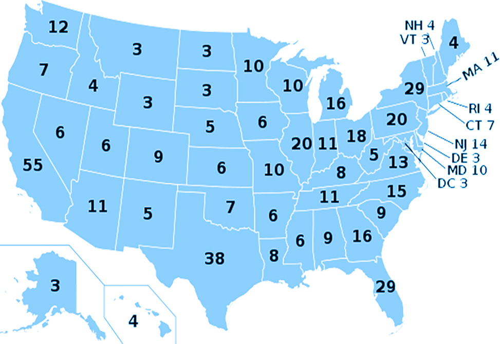

Benjamin Leinwand, Puyao Ge, Vidyadhar Kulkarni, Richard Smith¹

In two of the last five U.S. Presidential elections, the winner received fewer popular votes than his opponent. In 2000, George W. Bush received 47.9% of the popular vote to Al Gore’s 48.4%, and in 2016, Donald Trump received 46.1% to Hillary Clinton’s 48.2%. The remaining votes went to third-party candidates. The political implications of the disparity between popular vote share and electoral college outcomes have been discussed at length. The extremes of this phenomenon, however, have been examined less thoroughly. In both 2000 and 2016, the popular vote winner won by less than three percentage points, but would it be possible to lose the popular vote by, say, ten percentage points and still win the election? What about 20%? Whether you refer to this extreme outcome as “unfair” or “efficient,” it leads to the same question: what is the smallest percentage of the popular vote a candidate can garner while still winning the election?

This seemingly simple question can result in different answers depending on your assumptions about the universe of eligible voters, third-party vote share, and the percentage of truly “up-for-grabs” voters. The answer also hinges on the practically implausible scenario of one candidate winning several states by exactly one vote, and losing several others by the maximum possible margin. Though these outcomes are unrealistic, probing the boundaries may help us better understand the broader system.

First, let’s introduce how the electoral college works. While the US has 50 states, there are 51 territories of interest, as the 50 states and Washington, D.C. all have electoral votes which total to 538. Each territory gets a minimum of three electoral votes, with the rest of the 385 electoral votes assigned on the basis of population, DC cannot have more votes than any state – this caveat will come up later. Eight territories have the minimal three electoral votes, while California has 55. 49 territories² are “winner-take-all,” that is to say the winner of the popular vote in the territory gets all of the territory’s electoral votes, but for simplicity we treat all territories as winner take all, this doesn’t change the presented results. The candidate who wins at least 270 electoral votes becomes the next president. In theory, it is possible for a candidate to win with 269 electoral votes, in which case the tie would be split by a special vote of the House of Representatives, but this would be unprecedented and would almost certainly trigger further constitutional challenges, so we are ignoring this as a practical winning strategy. Nevertheless, we include percentages required to get to 269 electoral votes in parentheses to account for this possibility.

A number of previous articles have considered this extreme scenario. In particular, a report by National Public Radio, NPR³ published just before the 2016 election, described a scenario by which a candidate could win the election with just 23.1% of the popular vote, based on numbers of votes cast during the 2012 election. Their scenario was based on the successful candidate winning the following territories totaling exactly 270 electoral votes: Alabama, Alaska, Arizona, Arkansas, Colorado, Connecticut, Delaware, District of Columbia, Hawaii, Idaho, Indiana, Iowa, Kansas, Kentucky, Louisiana, Maine, Maryland, Massachusetts, Minnesota, Mississippi, Missouri, Montana, Nebraska, Nevada, New Hampshire, New Jersey, New Mexico, North Dakota, Oklahoma, Oregon, Rhode Island, South Carolina, South Dakota, Tennessee, Utah, Vermont, Virginia, West Virginia, Wisconsin, Wyoming. We have repeated the calculation using the same set of territories but based on 2016 voting numbers⁴, and based on the same assumptions, this could lead to a candidate winning 270 electoral votes with just 22.8% of the popular vote.

How did they find this supposedly optimal collection of territories? Well, their algorithm was really very simple. Take all the territories with the minimum 3 electoral votes, then add those with 4, then 5, and so on. They skipped Washington, 12 electoral votes, and substituted New Jersey, 14, because that made the total electoral votes exactly 270. Since the distribution of electoral votes has not changed since 2016, that could also be a winning combination for the 2020 election.

However, this Is not the optimal solution. Consider the following changes: from the above list, delete Alabama, Colorado, Iowa, Maryland, Massachusetts, Minnesota, Missouri, New Jersey, Oregon, Virginia and Wisconsin, replace by California, Georgia and Texas. Both the added and deleted territories total 109 electoral votes, so the 270 total remains unchanged, but based on the 2016 voting numbers, the successful candidate could have won with just 21.3% of the popular vote, about 1.5% of total votes fewer than the previous solution. If, instead, we took 269 electoral votes as the target, that percentage would be reduced even further, but only to 21.2%, with a different configuration of territories.

We used two approaches to verify that this is the optimal collection of territories. The first uses Monte Carlo methods, as described in Box 1. Algorithms of this nature have been used in the statistical literature, for example to find space-filling designs. Royle and Nychka⁵ discussed applications to the optimal construction of an environmental monitoring network, and also cited earlier applications of the same idea.

However, even with the Monte Carlo approach, it’s difficult to prove that the solution is optimal. From an optimization standpoint, the problem is an example of integer programming, as in Box 2, for which a number of computer packages now exist. Using IBM’s CPLEX Optimizer or the lpSolve function in R, we were able to verify that the same solution is obtained by integer programming.

This solution has some peculiar features beyond the assumptions about voting patterns that were used to derive it. The inclusion of California and Texas contradicts the common notion that the way to amass electoral votes is to win all the small territories, and it seems unlikely that both states would be won by the same party, since for decades California has been regarded as a Democratic stronghold with Texas just as strong on the Republican side. But perhaps that is part of the explanation why they feature in our optimal solution: both states have reduced turnout because they are regarded as a foregone conclusion, but that makes them more likely to be selected by our algorithm which favors states with a low ratio of popular votes to electoral college votes.

An alternative approach would be to base the analysis on “potential votes” in each territory, such as the total number of eligible voters. This is difficult to calculate precisely because different states have different rules of eligibility – noncitizens are barred from voting by federal law, and there are other restrictions such as convicted felons, that vary from state to state. Nevertheless, estimates of the “voting-eligible population,” VEP, as of the 2020 primaries are available at the state level4. For the moment, we assume that there are only two candidates and that all voters are “up-for-grabs.”

We will discuss more “realistic” extreme scenarios later in this article. Using VEP, a candidate could win the election, get 270 or more electoral votes, with only 22.2% of the popular vote, 22.1% if the candidate is only required to get 269 votes. This is based on the previous set of territories identified by NPR, deleting Colorado, Missouri and Virginia, 32 electoral votes, and adding Illinois and Washington, also 32. In contrast, if we used the NPR set of territories with this definition of voting population, the candidate could win with 22.4% of the vote, only very slightly higher. In all of these scenarios, however, it’s possible for a candidate to win with less than 23% of the vote.

Box 1: Monte Carlo Algorithm

A simple algorithm can be used to get a “good” solution, but can’t guarantee an optimal one. Let S be the proposed set of territories won by the election winning candidate, and let N be a large number, like 1 million.

1. Let S = all 51 territories.
2. Randomly choose integer K>0.
3. Randomly select K of the 51 territories.
4. Let S-new consist of S “swapping” all territories selected in step 3, those that were in S are removed; those that were not in S are added to S.
5. If S-new has either a) a larger population than S, or b) fewer than 270 electoral votes, reject the change and keep S. Otherwise, replace S by S-new.
6. Go back to step 2 and run steps 2 – 6 for N repetitions.

You can also run this algorithm several times and choose the best available result.

Box 2: Integer Program

An Integer Program, IP, is a constrained optimization problem where the decision variables are constrained to take integer values. An IP solver can provide a certificate that it has found an optimal solution, which is an improvement over the Monte Carlo Algorithm, but finding an optimal solution may take an extremely long time. Since there are only 51 territories, it is not computationally intractable to find optimal solutions to our problems using optimization software like CPLEX or SAS.

We can solve our initial problem with the following IP, which includes the “populations” and electoral votes in each territory as inputs.

Let: 1 ≤ i ≤ 51, representing each territory.

x(i) = 1 if the winner gets a majority of popular votes in territory i, 0 otherwise.

v(i) = Popular votes in territory i.

E(i) = Electoral votes in territory i.

We solve the following problem:

Minimize:

(x(1)v(1) + … + x(51)v(51))/2

Subject to:

x(1)E(1) + … + x(51)E(51) ≥ 270

and x(i) = 0 or 1, 1 ≤ i ≤ 51

Even the more complex problems we discuss do not require much more sophisticated IP formulations.

Constructing the Most Extreme Scenarios:

All the analyses so far have been based on the current distribution of electoral college votes. If we take into account possible redistributions of the US population and hence the numbers of electoral votes, far more extreme scenarios could arise.

At one extreme, suppose all the territories had equal populations and hence also equal numbers of electoral votes. Admittedly, that’s not exactly possible with 51 territories and 538 electoral votes, but we could construct scenarios very close to that. In such cases, it is possible for a candidate to win with just over 25% of the popular vote.

To define the opposite extreme, we first describe how electoral votes are allocated to each territory, called the Huntington-Hill method. The process is actually based on representatives and senators from each state, but for simplicity, we will explain how to get these values for the electoral college.

Each territory starts with three electoral votes. To distribute the remaining 385 votes, create a 51.385 table where each row represents a territory, and each column heading is calculated by the formula 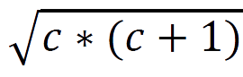, where c represents the column number. To get the value in each cell of the table, take the population of the corresponding territory and divide by the column heading. For each of the largest 385 values anywhere in the table, the territory in whose row the value resides gets an additional electoral vote.

For the lower bound, instead of splitting the population equally across all territories, we put a single person in 49 of the territories with three electoral votes each, and split the rest of the people between two gigantic territories. Using the Huntington-Hill method, allocate the remaining people so that the larger one will have 268 electoral votes, but is one person short of receiving 269 electoral votes. The rest of the people reside in the final territory, which must have 123 electoral votes. Additionally, assume all those ineligible to vote are in the second largest territory, so they count towards allotting electoral votes, but cannot contribute to the popular vote. The US reported a total population of 328,239,523 in 2019, but currently has an estimated 233,053,576 VEP, which leaves 95,185,947 people who are unable to vote. If 226,036,192 people who are all eligible to vote live in the largest territory, and 102,203,282 people live in the second largest territory, that leaves only 7,017,335 eligible voters in the second territory, one voter in all other territories, and crucially, gives the largest territory 268 total electoral votes. This allows the losing candidate to spend votes maximally disadvantageously, receiving no votes from all of the ultra-advantageous “one popular vote for three electoral votes” territories. If the electoral college loser wins all votes in the largest territory and just under half the votes in the second largest territory, that candidate would receive about 98.5% of the vote, leaving only 1.5% of the vote for the election winner. This calculation relies on the discrepancy between territories’ total populations, according to which electoral votes are allotted, and their voting eligible population, who can cast popular votes. If instead we ignore all non-eligible voters and reallocate electoral votes based on VEP, this same two territory packing method would allow the winner to receive just under 15.6%, 15.4%, of the popular vote.

For those eagle-eyed readers waiting for Chekhov’s caveat, there is one even sillier situation. If we packed the whole US population, minus 50 people – one for every state, into Washington, DC, by law, DC, cannot have more electoral votes than any state, so the votes would be split evenly across all territories. In that case, a candidate could receive only 26 votes – about one of every nine million eligible voters – and win the electoral college. Politically engaged readers may consider that this scenario could lead to increased calls for D.C. statehood, or perhaps secession.

Realistic Scenarios:

All the results presented so far are artificial: for example, no candidate will ever get 100% of the vote in any territory! However, we can also construct extreme scenarios that are more consistent with actual voter behavior.

We start by computing the smallest vote share each major party has received in any recent presidential election, whom we regard as “solid” Democrats and Republicans. The remainder are considered potential “swing voters.” We also incorporate the largest third-party vote share from the past several elections, or equivalently, the largest percentage of votes that went to neither of the two major parties. Sometimes, third-party candidates attract a substantial percentage of the vote in a given state, for example, in 2016 in Utah, independent Evan McMullin captured 21.5% of the vote, not far behind Hillary Clinton’s 27.5%. As recently as 1992, independent Ross Perot received 18.9% of the national vote and may well have been responsible for Bill Clinton’s victory that year. Clearly, constructing more realistic scenarios needs to take account of third-party candidates.

With these broader assumptions, we now slightly change the question to “what is the largest percentage of the popular vote by which a candidate can lose while still winning the election?” We are still assuming the ultimate winner is from one of the two major parties, but allowing, for example, that if a third-party candidate in some territory gets 20% of the vote, that makes it possible for a major-party candidate to win the territory with only just over 40% of the votes in that territory.

We use the most extreme statewide results from recent elections as a proxy for each party’s support floor and maximal third-party vote share in each state. One calculation uses the five elections between 2000 and 2016, as these elections have had relatively small national third-party vote shares. For the second case, we also include 1996 and 1992. The most extreme achievable results based on these different assumptions, as well as the choice of population, are presented in the table below. Not surprisingly, given Perot’s performance in 1992, the results that include that year are more extreme.

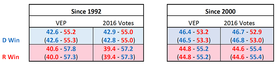
In all these scenarios, Republicans can win the election with getting fewer votes than Democrats could. The distributional characteristics of the electorate that have enabled Republicans to win two elections while losing the popular vote this century also feature in these calculations. Still, even with “conservative assumptions,” it is also possible for a Democrat to win the election while losing the popular vote by more than six points.

In this article, we have presented numerous scenarios, with varying degrees of plausibility, that show how it is possible to win the US presidential election with a minority of the popular vote. Of course, one simple change in the rules would make all our scenarios not merely implausible, but actually impossible: change the law so that the winner of the national popular vote becomes the president.

Footnotes

1 Benjamin Leinwand and Puyao Ge are graduate students, and Vidyadhar Kulkarni and Richard Smith, are professors in the Department of Statistics and Operations Research, University of North Carolina, Chapel Hill, NC, USA. The authors would like to thank Professor Gabor Pataki for advice about integer programming. Email address for correspondence: rls@email.unc.edu. The authors declare that they have no competing financial interests.

2 Maine and Nebraska assign one electoral vote to the winner of each of their districts (two in Maine, three in Nebraska), and their remaining two electoral votes go to the statewide popular vote winner. The historical data necessary for calculating the realistic scenarios could not be found at the district level, so for only those scenarios, comparisons could not be made between the two sets of rules.

3 LINK

4 LINK

5 Royle, J.A. and Nychka, D., 1998, An algorithm for the construction of spatial coverage designs with implementation in S-PLUS. Computers and Geosciences 24(5), 479-488